OpenSees coming to python!

One of the gripes a lot of people have with OpenSees is that it adopts TCL as its interpreter language. Originally, OpenSees was conceived as a framework, this is apparent from the main page of the wiki:

OpenSees, the Open System for Earthquake Engineering Simulation, is an object-oriented, open source software framework. It allows users to create both serial and parallel finite element computer applications for simulating...

So, it was meant to be a neat way to build new FEM software. For years the only actual (known) application to use the OpenSees framework was what came to be known as OpenSees proper, a TCL interpreter extended with OpenSees modeling commands. Talking with Frank McKenna, the mind behind OpenSees, this stemmed from then need to show an actual application which could demonstrate the idea of the OpenSees framework in a quick and dirty way. The vision was that people would get the OpenSees source and build new and exciting finite-element software. It was "up to the skills of the user", like the main wiki page still reads.

Sadly, civil engineers are not very code-savvy and no (useful) new applications came. Therefore it came to pass that the OpenSees extension of the TCL interpreter became OpenSees and this is what everyone uses.

Now TCL is an awkward language for a scientific application, mainly due to syntax and lack of a complete library for scientific computing. Python, on the other hand, has proven in the recent years to be a worthy replacement of the mighty Matlab. Many of us started scientific computing in Matlab and then migrated to the free world of Python. It was just logical that OpenSees would benefit much more from using Python as its language of choice rather than TCL.

It has finally happened, and this blog post celebrates my joy. Behold the following analysis case written in Python.

import opensees as ops

ops.wipe()

ops.model('basic', '-ndm', 3, '-ndf', 3)

for e in range(3):
    ops.node(1+4*e, 0., 0., 1.*e)
    ops.node(2+4*e, 1., 0., 1.*e)
    ops.node(3+4*e, 1., 1., 1.*e)
    ops.node(4+4*e, 0., 1., 1.*e)

ops.fix(1, 1, 1, 1)
ops.fix(2, 1, 1, 1)
ops.fix(3, 1, 1, 1)
ops.fix(4, 1, 1, 1)

ops.nDMaterial("ElasticIsotropic3D", 1, 2100., 0.3, 0.0)

ops.element("stdBrick",1,1,2,3,4,5,6,7,8,1)
ops.element("stdBrick",2,5,6,7,8,9,10,11,12,1)

ops.timeSeries("Linear", 1)
ops.pattern("Plain", 1, 1, "-fact", 1.0)
ops.load(1+4*e, 0., 0., -50.)  # Load at the first of the top nodes.

ops.system("BandSPD")
ops.numberer("RCM")
ops.constraints("Plain")
ops.algorithm("Linear")
ops.integrator("LoadControl", 1.0)
ops.analysis("Static")
ops.analyze(1)

This example just stacks two bricks and applies a downward load on one of the top nodes. The interesting part is that now you can interact with all of the rich tools available in python. Just as a taste of what's to come, here is a plot of the deformed shape of the example above created using matplotlib's 3-D plotting capabilities.

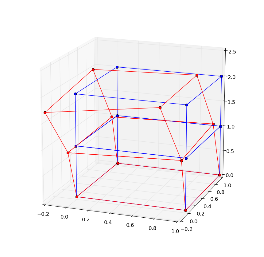
And here's the code that achieves this:

### Plot bricks in the domain
import scipy as sp
import matplotlib.pyplot as plt
from mpl_toolkits.mplot3d import Axes3D
fig = plt.figure()
ax = fig.add_subplot(111, projection='3d')

for e in ops.getEleTags():

    nodes = ops.eleNodes(e)
    Nnodes = len(nodes)

    xyz = sp.zeros((Nnodes,3), dtype=sp.double)
    uu   = sp.zeros((Nnodes,3), dtype=sp.double)
    for i in range(Nnodes):
        xyz[i,:] = ops.nodeCoord(nodes[i])
        uu[i,:] = ops.nodeDisp(nodes[i])

    print

    x = sp.zeros(12,dtype=sp.double)
    y = sp.zeros(12,dtype=sp.double)
    z = sp.zeros(12,dtype=sp.double)
    u = sp.zeros(12,dtype=sp.double)
    v = sp.zeros(12,dtype=sp.double)
    w = sp.zeros(12,dtype=sp.double)

    conec = [0, 1, -1, \
    1, 2, -1,\
    2, 3, -1,\
    3, 0, -1,\
    4, 5, -1,\
    5, 6, -1,\
    6, 7, -1,\
    7, 4, -1,\
    0, 4, -1,\
    1, 5, -1,\
    2, 6, -1,\
    3, 7
    ]

    x = xyz[conec,0]
    y = xyz[conec,1]
    z = xyz[conec,2]
    x[2::3] = sp.nan
    y[2::3] = sp.nan
    z[2::3] = sp.nan

    factor = 1.
    u = xyz[conec,0] + factor*uu[conec,0]
    v = xyz[conec,1] + factor*uu[conec,1]
    w = xyz[conec,2] + factor*uu[conec,2]
    u[2::3] = sp.nan
    v[2::3] = sp.nan
    w[2::3] = sp.nan

    ax.plot(x,y,z,"-ob")
    ax.plot(u,v,w,"-or")
plt.show()

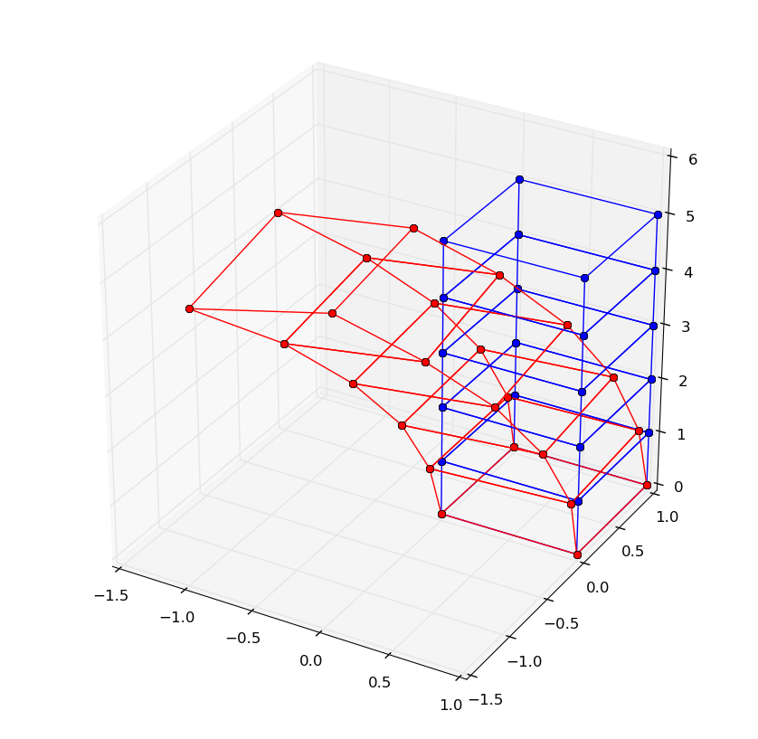
A simple extension to the above example generalizes the stack to an arbitrary number of bricks. And the visualization just works.

Currently, I have to manually compile a python module extension on my Ubuntu linux laptop for this to work. I have no idea if it will be available to windows users as an easy-to-download binary in the near future. I will post on how to get this working on linux though. For those of you adventurous enough.