SNE # 0. Stochastic inverse pendulum
This is the first installment of "Small Numerical Experiments" (SNE), a section where I upload and comment (briefly) some small numerical example. The purpose is to prove a point to myself, test some code, ideas, etc.
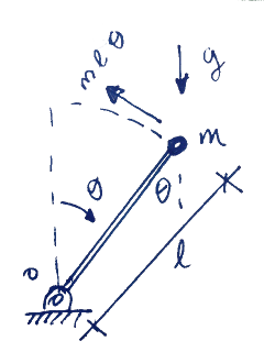
In this first post I will explore the response of a stochastic inverse pendulum. What I mean in this case is an inverse pendulum (shown left) with a random initial condition. The purpose is to obtain the time-evolving probability density function (PDF) of the pendulum's position. I will be doing Monte-Carlo simulations to obtain an approximation to this PDF.
The response of the system is governed by the following nonlinear ordinary differential equation in terms of the angular displacement $\theta$ with respect to the vertical:
$$ m l^2 \ddot{\theta} + c \dot{\theta} - mgl \sin \theta = 0 $$
Subject to an initial condition $$ \theta(0) = \theta_0$$ and $$ \dot{\theta}(0) =\dot{\theta}_0$$. In this case, the initial angular velocity is set to zero and the initial angular displacement is set to have a Gaussian random distribution with mean zero and standard deviation of 10 degrees. The linear damping constant is set to 10% critical damping the system would have in the case of small oscillations about the final equilibrium point $$\theta = 180^{\circ}$$.
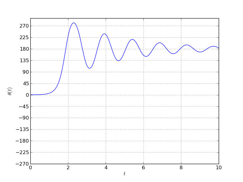
The example is coded in python and solved using the odeint solver available in scipy. Here is an example response for a given nonzero initial condition.
Doing 5000 Monte-Carlo draws and plotting all the responses together we
get: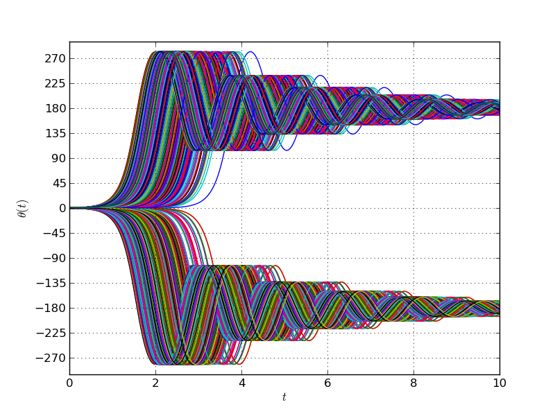
-About half of the the pendulums swing to the left and the other half to the right. This would result in a bimodal distribution and is a mere artifact of the mathematical model used. Indeed, what the model perceives as two distinct equilibrium points are actually the same position for the pendulum. This arises because of the periodicity in the $\sin()$ function.
From this set of motions a PDF may be computed for each time and animated to show the evolution of the PDF with time.
The bimodal distribution obtained at the end is, therefore, an artifact, as the peaks correspond to the same final configuration for the system. In a more complex case it might not be possible to distinguish between peaks in PDFs which are real, ie. correspond to physically different configurations, from those that arise from deficiencies in the mathematical tool used.
These spurious peaks generate unrealistic dispersion in the distribution of results. Is there a way to identify them and get rid of them?
The following python code produces these results.
#!/bin/python
# -*- coding: utf-8 -*-
# Small numerical experiments # 00
"""
@SNE_number: 00
@Title: Stochastic inverse pendulum
@Idea: Show a case in which bifurcation behavior produces multimodal
distribution.
@Tags: scipy, ode, stochastic, multimodal, bimodal, matplotlib,
Monte-Carlo, animation, python
@Date: Created on Fri Oct 4 2013
@author: jaabell
"""

import scipy as sp
import matplotlib.pylab as plt
from scipy.integrate import odeint

N = 5000 #[] number of Monte-Carlo trials
mu_theta = 0.0 #[deg]
sigma_theta = 10 #[deg]
tmax = 10 #[s] Maximum time for simulation
dt = 0.01 #[s] Time step for integration
m = 1 #[]
g = 9.81 #[m/s\^2]
l = 0.50 #[m]
xi = 0.3 #[] Ratio of critical damping (for a regular pendulum under
small deflections)
Nbins = 50 #[] Number of bins for computing histograms
theta_0_dot = 0.0 #[deg/sec] initial angular velocity for pendulums

compute = False #Use this in an interactive session (ie. spyder) to
avoid recomputing the Monte-Carlo runs

c = 2*xi*m*l**2 #[N*m*s/rad] Damping constant
Nt = int(tmax/dt) #[] Number of simulation timesteps

#Generate parameters for Monte-Carlo trials
mu_theta_rad = mu_theta*sp.pi/180
sigma_theta_rad = sigma_theta*sp.pi/180
thetas = sp.randn((N))*sigma_theta_rad + mu_theta_rad
t = sp.arange(0,tmax, dt)

#Recast problem as a set of first order ODEs
b = -c/(m*l**2)
a = g/l
def func(y, t):
    return [y[1],a*sp.sin(y[0]) + b*y[1] ]

def gradient(y,t):
    return [[0.0,1.0],[a*sp.cos(y[0]),b]]

#Do the Monte-Carlo runs
if compute:
    yall = sp.zeros((Nt,N))
    i = 0
    for theta_0 in thetas:
        y0 = [theta_0*sp.pi/180, theta_0_dot*sp.pi/180]
        y = odeint(func, y0, t, Dfun=gradient)
        yall[:,i] = y[:,0]
        print "Case {} of {}".format(i,N)
        i+= 1

# Some plotting (animation after a tutorial found in http://jakevdp.github.io/blog/2012/08/18/matplotlib-animation-tutorial/)
# Also look at http://matplotlib.org/api/animation_api.html
plt.close("all")

from matplotlib import animation

# First set up the figure, the axis, and the plot element we want to
animate
fig = plt.figure()
ax = plt.axes(xlim=(-300, 300), ylim=(0, 10))
ax.grid()
ax.set_xticks(sp.linspace(-270,270,num=7))
ax.set_xlabel("$\\\theta$")
ax.set_ylabel("$f_{\\\theta}(\\\theta, t)$")

line, = ax.plot([], [], lw=2)

time_text = ax.text(-270, 9, '')#, transform=ax.transAxes)

from scipy.interpolate import interp1d
probability_thresholds = sp.linspace(0,1,21)

def myhistogram(y):
    yn = sp.array(y)
    yn.sort()
    cdf = sp.linspace(0,1,yn.size)
    y_bins = interp1d(cdf, yn, kind='linear', axis=-1, copy=True,
    bounds_error=True)(probability_thresholds)
    return probability_thresholds, y_bins

def init():
    line.set_data([],[])
    time_text.set_text("")
    return line, time_text

def animate(i):
    cdf, y_bins = myhistogram(yall[i,:])
    pdf = sp.diff(cdf) / sp.diff(y_bins)
    y_bins_centers = 0.5*(y_bins[0:-1] + y_bins[1::])
    # pdf, y_bins = sp.histogram(yall[i,:], bins = Nbins, density =
    True)
    # y_bins_centers = 0.5*(y_bins[0:-1] + y_bins[1::])
    line.set_data(y_bins_centers*180/sp.pi, pdf)
    time_text.set_text("Time = {0:4.2f} s".format(t[i]))
    return line, time_text

anim = animation.FuncAnimation(fig, animate, init_func=init,
frames=1000, interval=1, blit=True)
#anim.save('basic_animation.mp4', fps=30, extra_args=['-vcodec',
'libx264'])

plt.show()

#plt.figure()
#plt.plot(t,yall[:,0]*180/sp.pi)
#plt.grid()
#plt.yticks(sp.linspace(-270,270,num=13))
#plt.xlabel("$t$")
#plt.ylabel("$\\\theta(t)$")